To see previous post click here. This time I will cover how I created all the parts of the G-V.
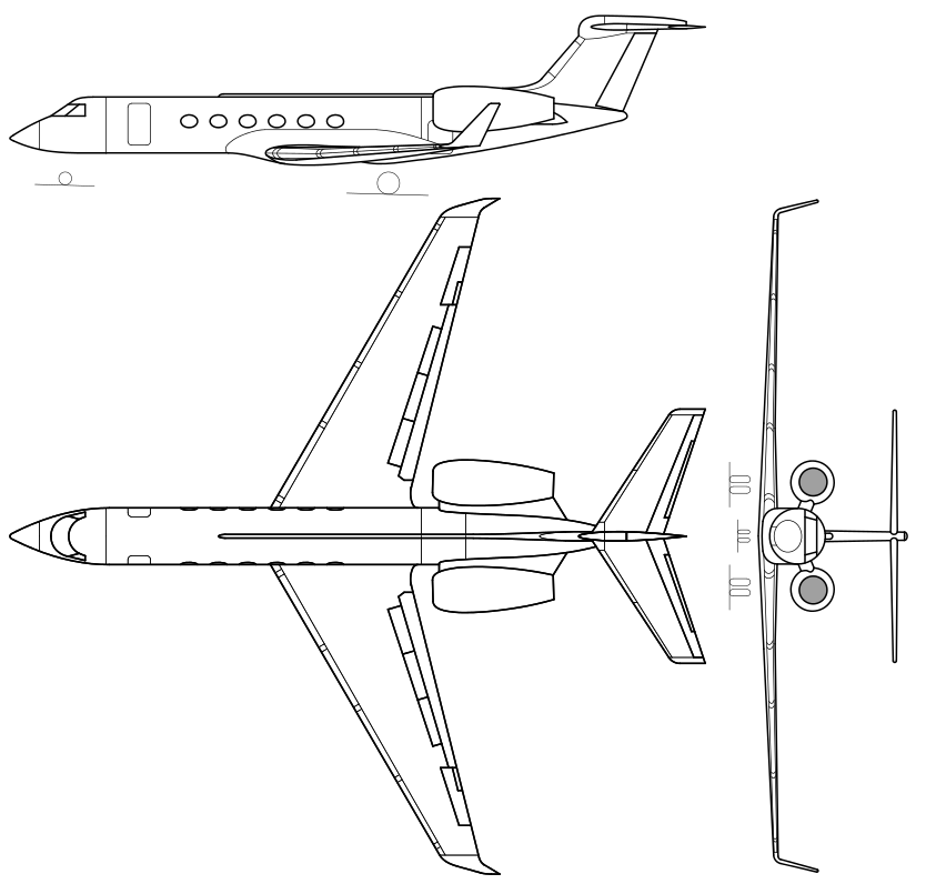
It pays to read all the way through. Last week, I thought that I had found technical drawings showing all the dimensions of the G-V. What I had actually found was a drawing describing taxi clearance.
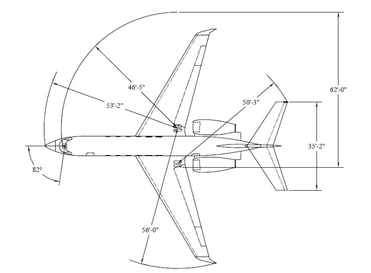
Drawing courtesy of NSF/NCAR and Lockheed Martin
So… back to the drawing board. Excuse the pun.
I divided the G-V into 4 parts: wing, fuselage, empennage, and engine. The more I separate the easier it makes it on me to get the details right.
Wing:
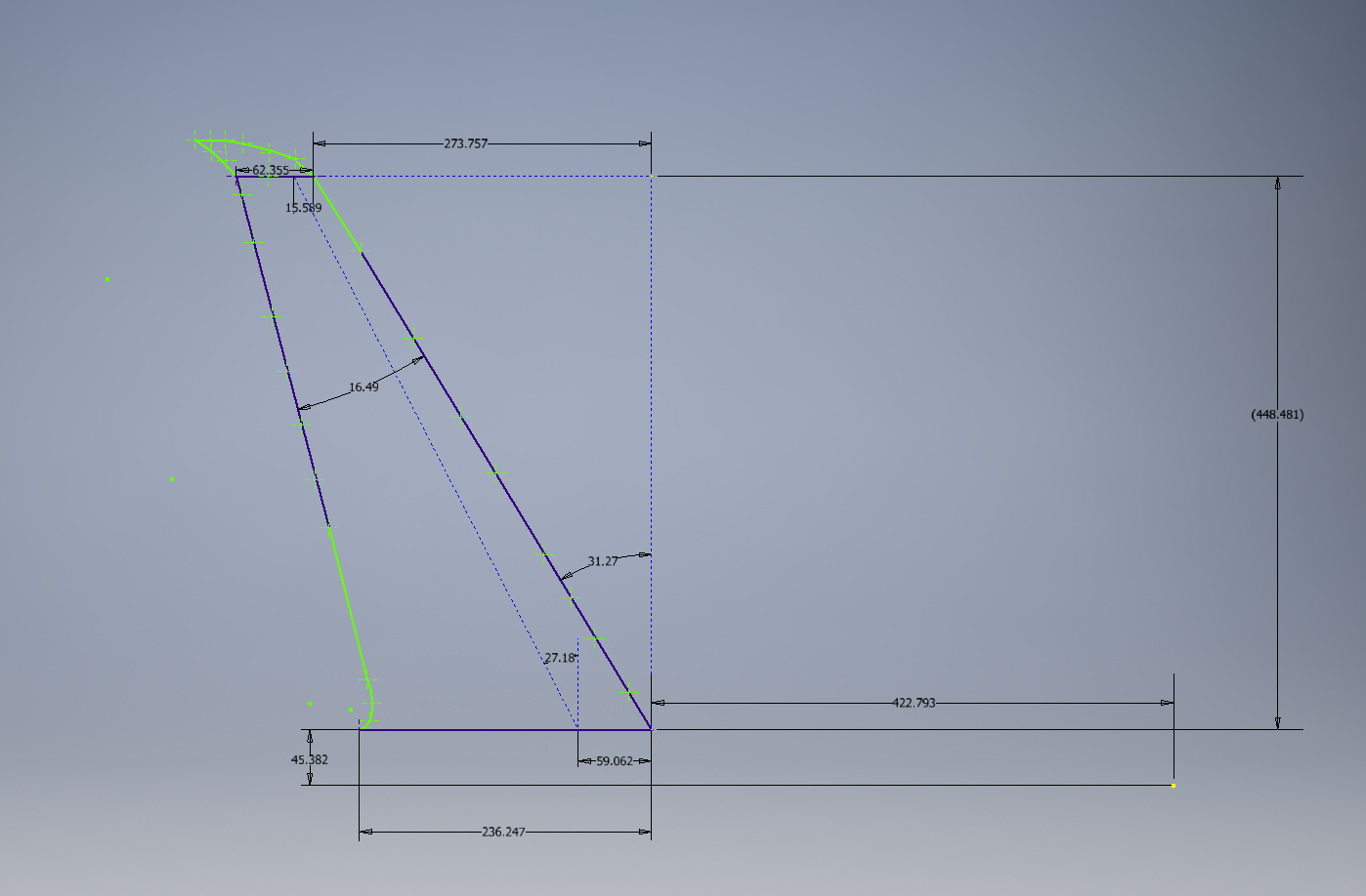
Going back to our Investigator Handbook from the NSF/NCAR we use a different technical drawing. In 5.1.5 of the handbook the pylon mounts along the wing for scientific investigation are shown. Using WebPlotDigitizer we create a series of points approximating the top of the wing. You have the option to save the points as a .CSV. Since I use Autodesk Inventor I can import Excel files with a series of data points. There are similar features with SolidWorks but I’m more comfortable with Inventor.
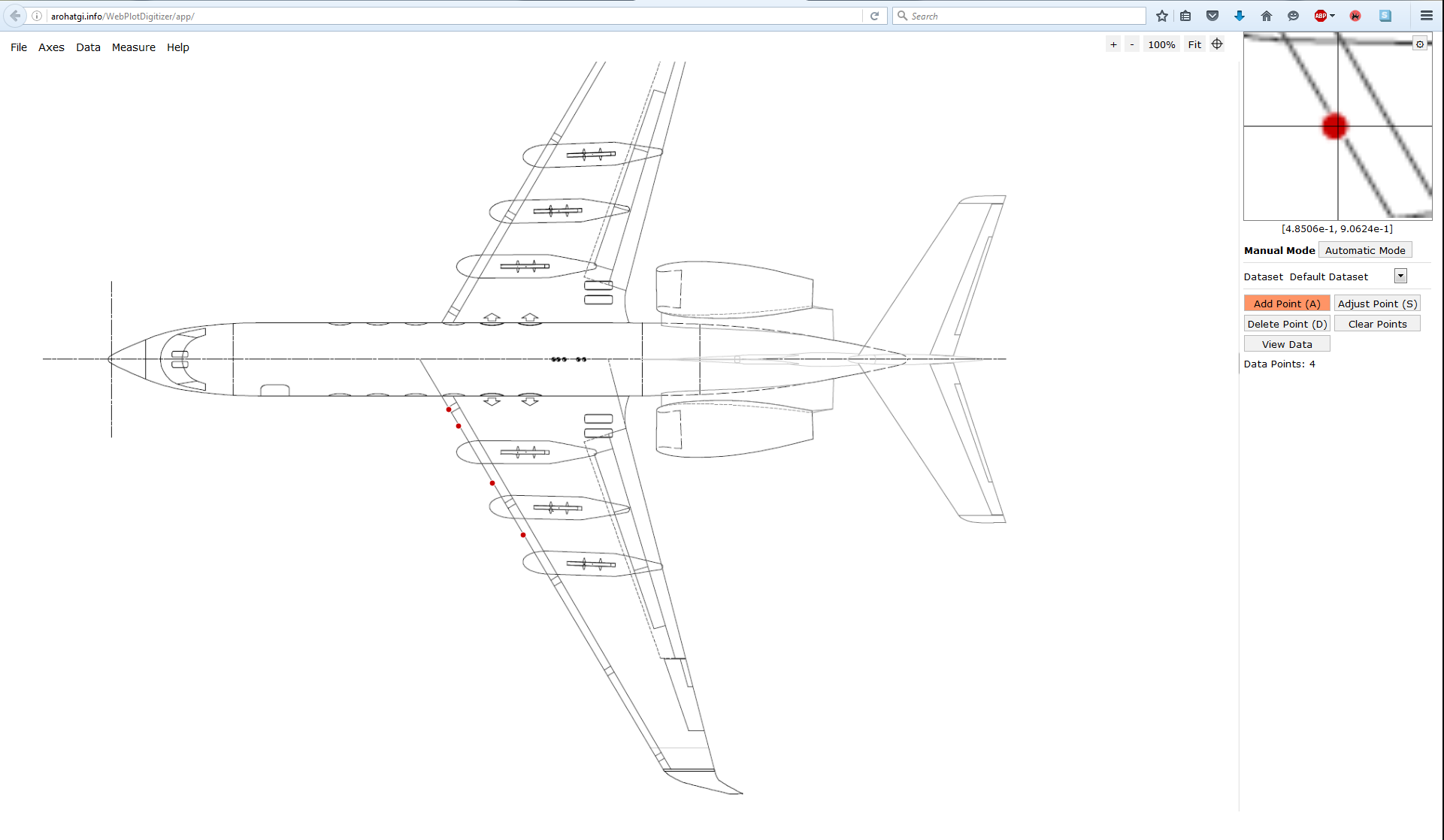
Once in Inventor I can begin making the wing. It’s almost connect-the-dots: except you need to check dimensions. You won’t have gotten all your points in the plot digitizer just right either so you should focus on getting the majority of the points as opposed to every single one. With more experience you’ll find that the more points you have on a curved surface the closer you can approximate the curve. The c⁄4 angle is 27° which is verified through the use of construction lines.
Now we have a sketch how do we create our 3D model?
Using the excellent resource The Incomplete Guide to Airfoil Usage we can determine the airfoils used for the root and tip of the wing. This provides us with the G-IV root airfoil, NACA 0012 modified, and the tip airfoil, NACA 64A008.5 modified.We don’t need to worry about the modifications or that it is G-IV because we’re developing a base model for concept development. The G-IV airfoils are essentially the same as the G-V anyways. If you were trying to get the airflow characteristics of a G-500 to the 99th percentile then you are either working for Gulfstream and can pull the model yourself or you should contact Gulfstream.
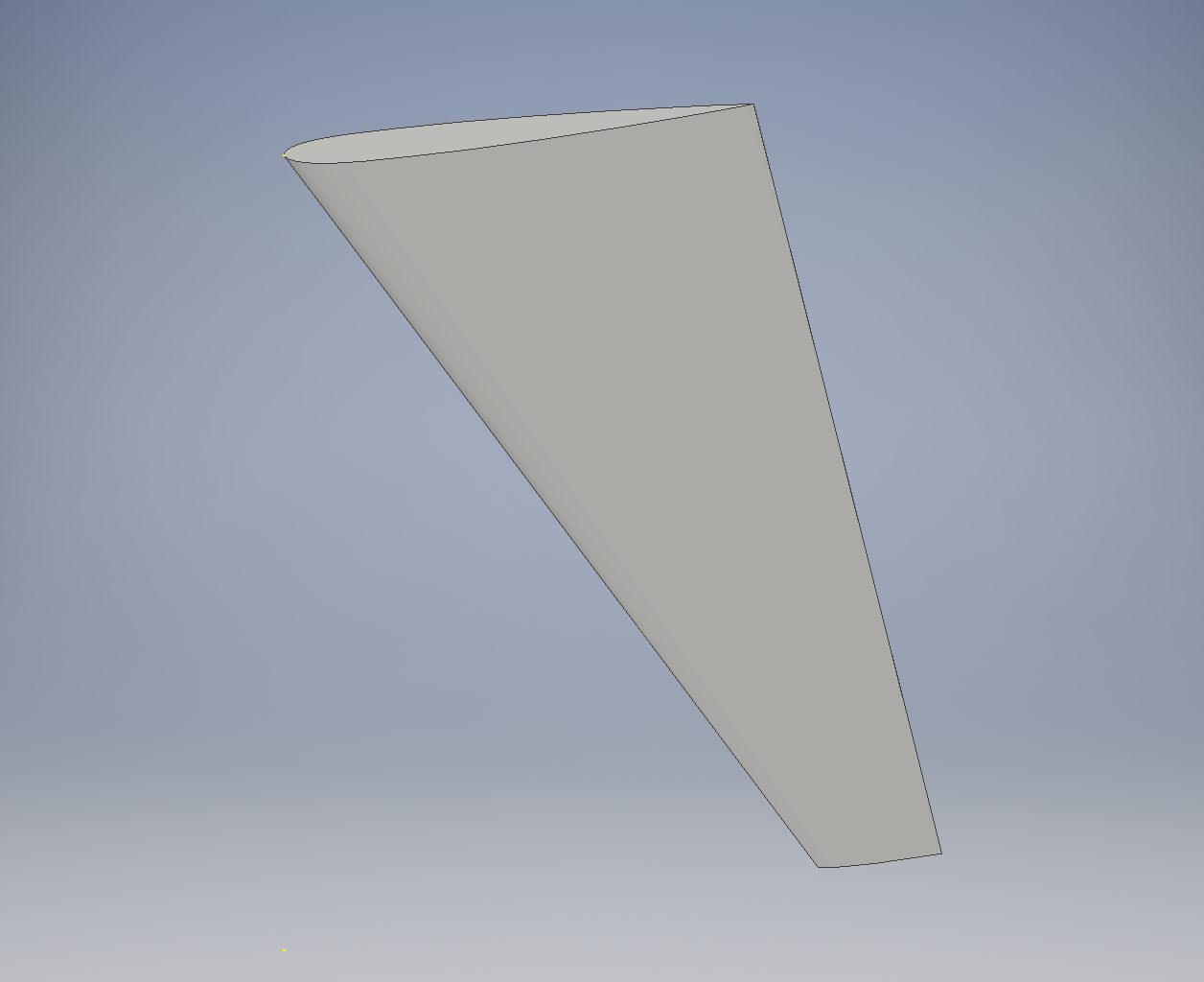
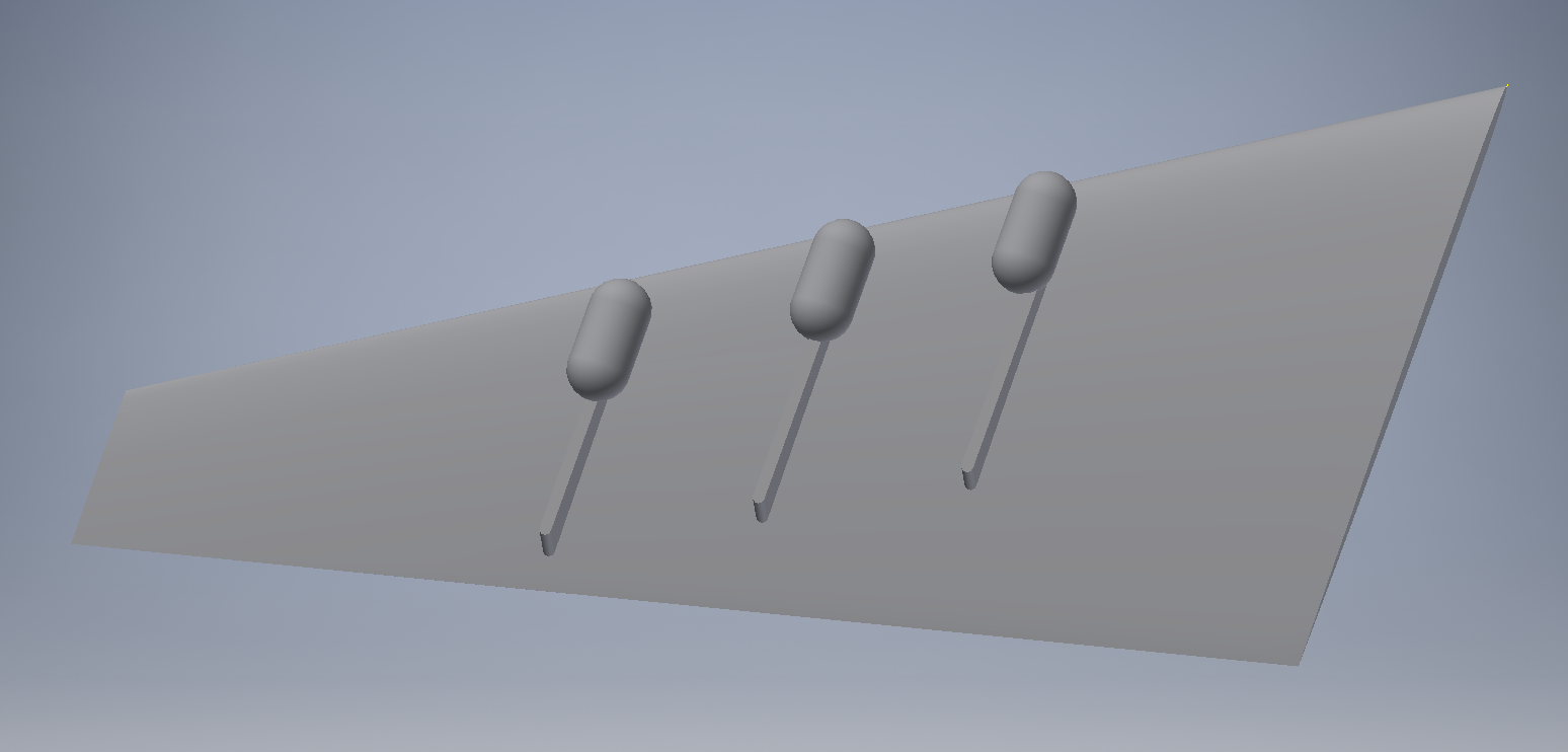
Using the 2D sketch we just created we can place the airfoils at their respective locations and loft the wing between them. That should give you something like this:
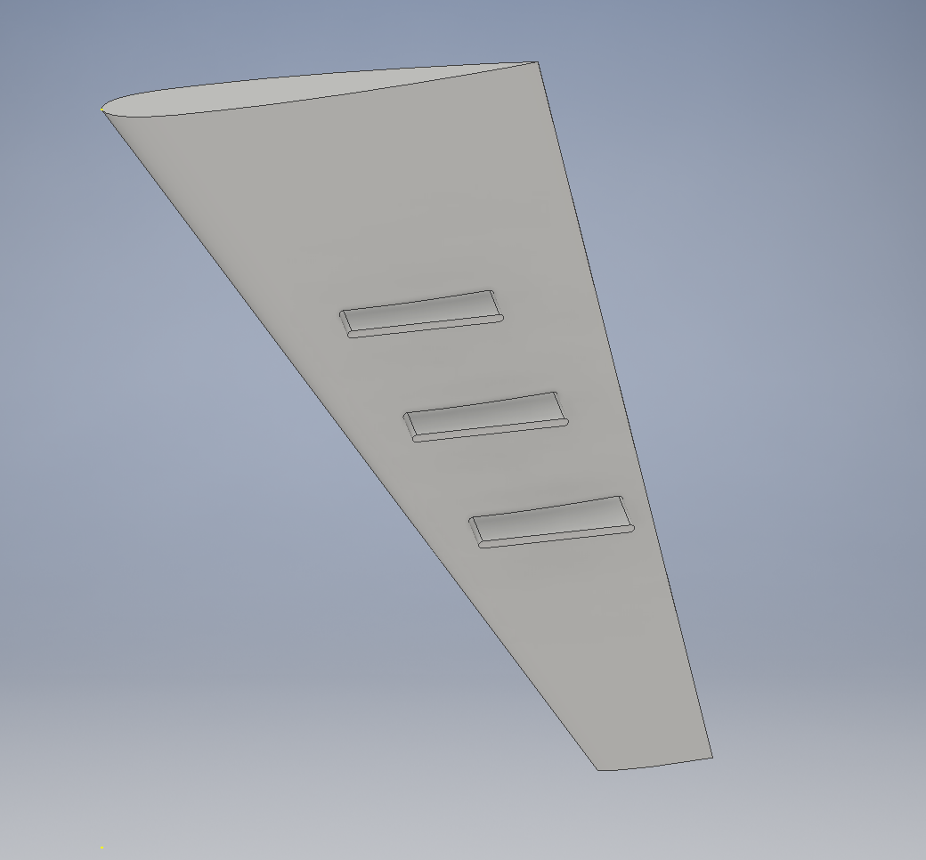
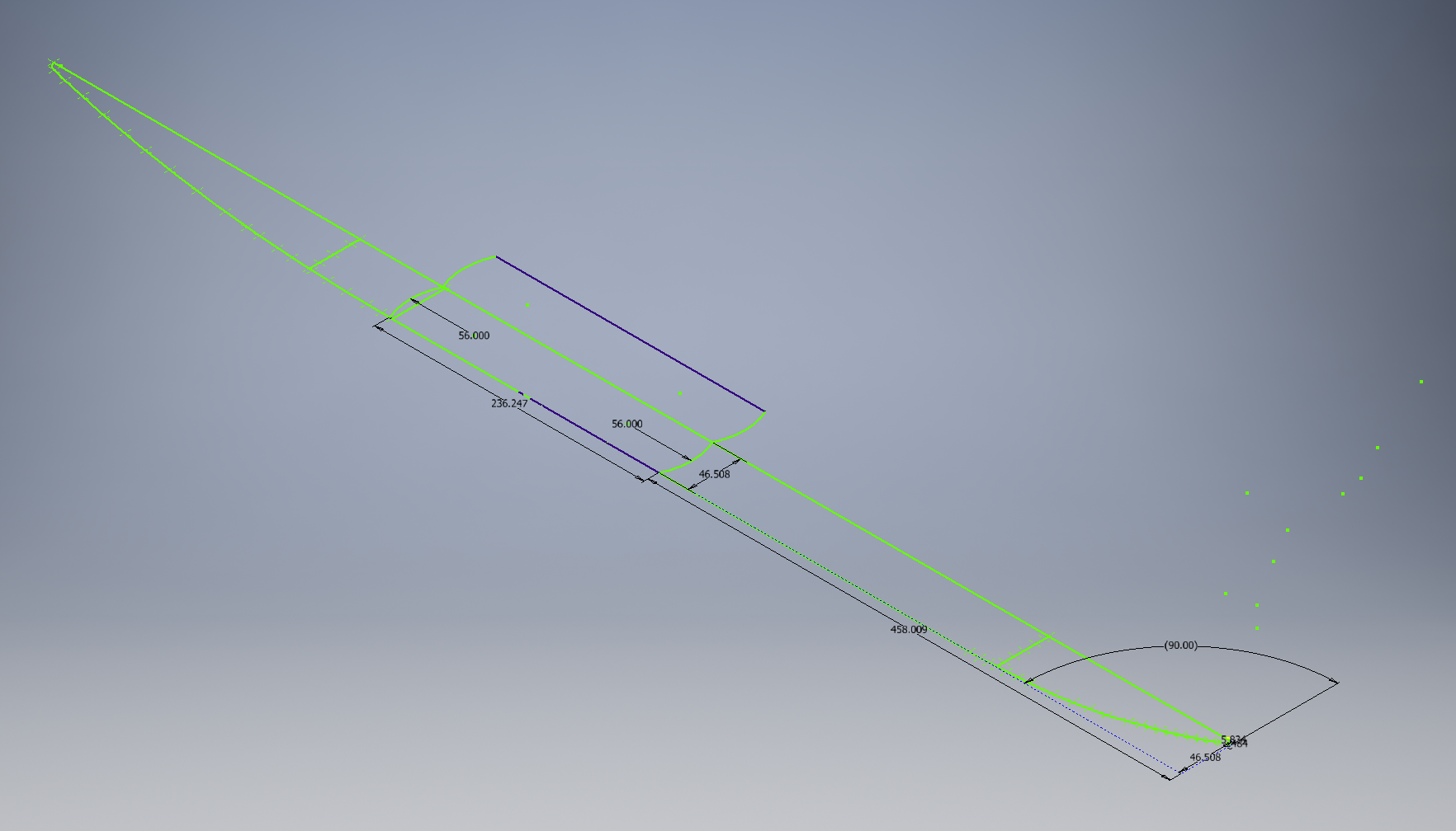
Then, using the sketch, which I hid in the previous image, create a work plane and extend your pylons in the appropriate locations.
I have a concept structure that I’m developing below. Currently, Dr. O’Neill is trying to provide Dr. Yan with some feedback on design of radio antenna integration for a Gulfstream G-V and I’m creating the CAD concept models. I cannot picture these currently because it’s ongoing research. Instead here are some example tank concepts.
Example Concept
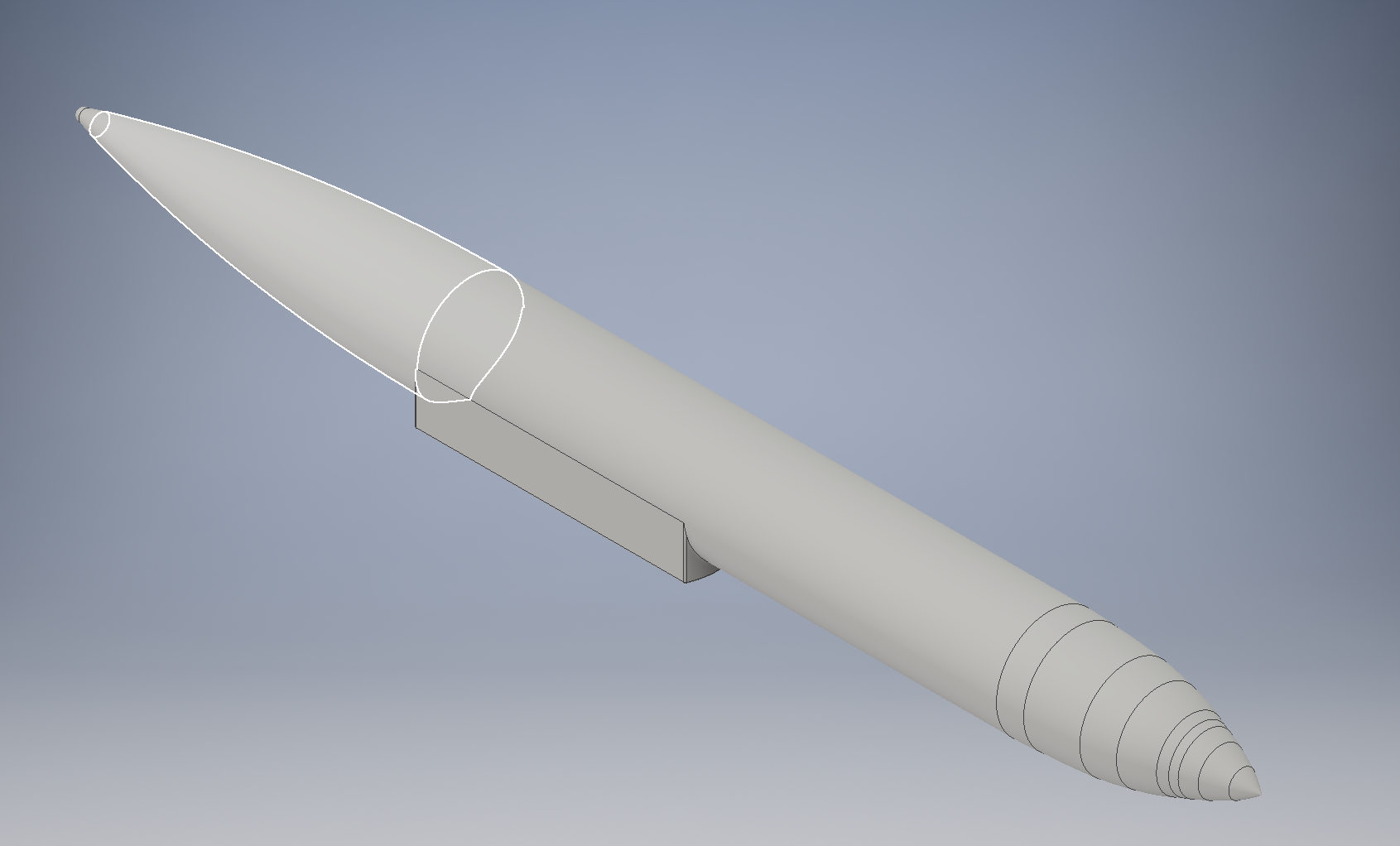
Fuselage:
The fuselage is created in a similar process to the wing. We plot a series of points and rotate the fuselage around the centerline. We will create the saddle with straight sides and extend it through the fuselage. The trick here is that I created 2 different sketches on the same plane to avoid weird things that happen if I make the pieces sequentially.
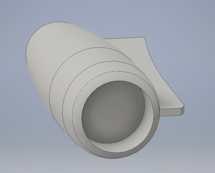
Rolls-Royce BR710A1-10 Turbofan Engine:
The Rolls-Royce engine is built in the exact same way as the fuselage. Two sketches on top of each other and then a rotation and an extension. I then cut into the engine to make it look like an actual engine but if you know how to extend by know this should be an easy process.
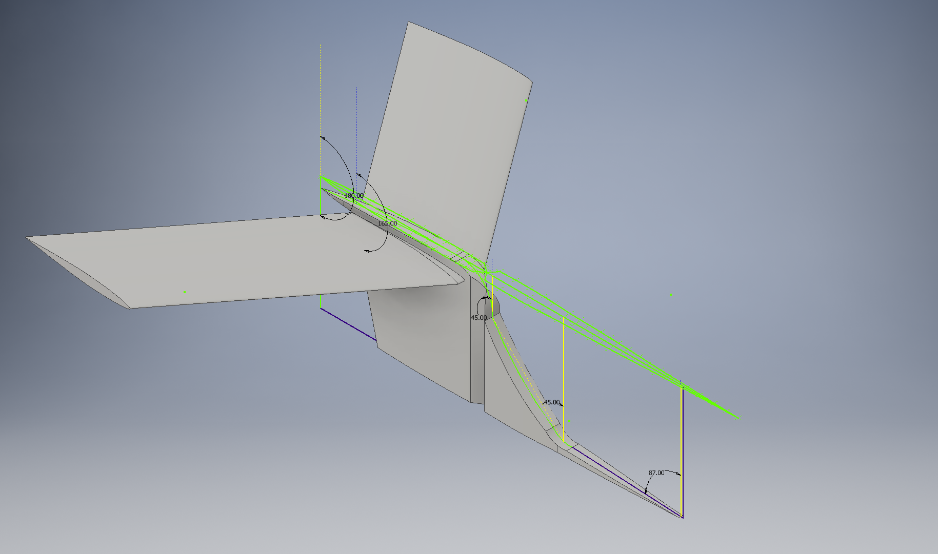
Empennage:
The tail is created by taking the points from the top view. The points are extended and then cut from the side view. The wings are lofted from the vertical stabilizer using the NACA 64A008.5 airfoil for the root and tip.
Complete Gulfstream G-V:
The current configuration of the Gulfstream is shown below. The illustrations shown are from the presentation I created for Dr. Yan. The antenna configuration is removed. Inventor has some nice illustration tools that are exceptionally useful when presenting.
The slideshow shows the stages of development of the Gulfstream G-V. The first model is all one piece. The second model is a lofted fuselage that experienced connectivity issues. The third is the most promising and will probably stay until I need to create updates for higher fidelity. The higher fidelity will be required when we run the antenna configuration through CFD to test the drag force produced by the array. As you can see I abandoned the wingtips until I have the antenna array configuration fixed.