Tag Archives: Academic

Specific Energy of an Orbit

Specific Energy for a Two-Body Orbit

Specific energy for a two-body orbit will be derived below. Specific energy of an orbit is constant in the two-body system. To further refine our definition, we are concerned with conservative forces only. This way specific mechanical energy is an exchange between potential and kinetic energy without drag or other perturbation losses that are non-conservative.

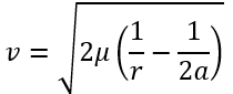
Specific energy was provided without proof in Eq. (1), from the previous article, "Orbital Speed for All Conic Sections," reproduced below.
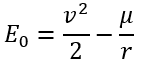
(1)

Specific energy is further reduced for all conic sections in Eq. (2) as a function of the gravitational parameter for the central body and the semimajor axis of the orbit.

(2)

Specific Energy Derivation

Given the two-body equation of motion, Eq. (3) we derive the specific energy for all conic orbits.
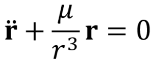
(3)

Step 1: Multiply by r-dot

Rearranging and multiplying by the derivative of position with respect to time,

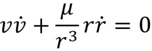
Step 2: Replace with derivatives of KE and PE w/r to time

As the scalar velocity multiplied by the scalar derivative of velocity term is equivalent to the derivative of kinetic energy with respect to time, we replace it as shown below on the left-hand side. The derivative of potential energy or the gravitational parameter over the radial distance is equivalent to the gravitational parameter over the radial distance squared multiplied by the scalar derivative of the position. To make the term general, we include the constant, c, which physically represents where we draw the datum for potential energy.

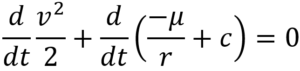
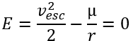
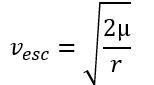
Step 3: Set the reference for PE to 0 (reference level at infinity)

Setting the constant, c, to zero is equivalent to setting the datum for potential energy at infinity.

(1)

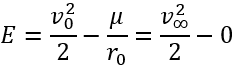
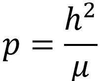
Function of semimajor axis and gravitational parameter

Using the periapsis and semilatus rectum's relationship to the specific angular momentum and gravitational parameter, the specific energy can be reduced to Eq. (2).
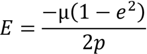
(2)

The semimajor axis is positive for circular and elliptic orbits, infinite for a parabolic orbit, and negative for a hyperbolic orbit. Thus, the energy of each is negative, zero, and positive, respectively.

Specific energy for conic sections rearranged to determine orbital speed.

Orbital Speed for All Conic Sections

Specific Energy for Two-Body Orbit

Specific energy is provided, without proof, in Eq. (1) for where specific energy is a constant for any conic section. Derivation will be provided in future articles.

(1)

Specific energy is further reduced for all conic sections in Eq. (2) as a function of the gravitational parameter for the central body and the semimajor axis of the orbit.

(2)

Orbital Speed for All Conic Sections

Elliptical and Circular

Using the specific energy equations (1) and (2), we can calculate the speed at some distance, r, from the focus as shown in Eq. (1).

(3)

There is no variation in the distance from the focus in a circular orbit, . Reducing Eq. (3) to Eq. (4), we only need to know the circular orbit radius and gravitational parameter of the central body. The circular orbit radius is equal to the semimajor axis.

(4)

Parabolic

A parabolic orbit represents the line between closed and open conic orbits. A probe given sufficient escape speed will travel on a parabolic escape trajectory from the central body. As the probe’s distance from the central body increases the speed necessary to escape decreases to zero. We determine the escape speed by comparing the specific energy of two points along this theoretical escape trajectory.

(5)

Hyperbolic

Using the same trick as a parabolic orbit for the hyperbolic orbit, we must account for the excess hyperbolic speed at some infinite distance.

(6)

Marshall Space Flight Center Fiscal Year 2019 Student Collaboration Projects (SCPs) – SIMPSON

Want updates?

Visit the project page for the most up-to-date information!

NASA Marshall Space Flight Center (MSFC) released a call on June 3 for proposals to collaborate with promising students and leverage ongoing work to explore new, innovative applications of that ongoing work.

Executive Summary

Christopher Simpson will build a 130-430 MHz dual-use software-defined radio to test inter-formation networking and precise navigation and timing. This device will later use 24-GHz Ka-band to allow data-rates of 1-Gbps. The prototype will be presented in March 2020 at the conclusion of the effort. The payload functions as a passive radar and directed beam by utilizing electronic beam-forming, passive illumination, and network time reference protocols. During AY 2019-2020, 2 demonstration nodes will be built to test this game-changing technology in formation flying.

Mr. Simpson intends to collaborate with Marshall Space Flight Center researchers developing inter-CubeSat communication using a peer-to-peer topology. The mesh network architecture MSFC researchers are developing is intended to allow for data exchange between spacecraft with no central router. The waveform currently in use will be leveraged to reduce development risk.

This proposal addresses NASA Roadmap 2015 - TA 5.5.1.1, Intelligent Multipurpose Software Defined Radio and enhances a return to the lunar surface by addressing LEAG - Strategic Knowledge Gap (SKG) Theme 1-D Polar Resources 7.

Addressing the Scientific and Technical Challenges

1.Track and communicate with other nodes (Satellites in the formation)

  • Simulate on ground the tracking and communication capability this network will provide

2.Expanding Network Time Reference (NRT) to communication systems to reduce reliance on external time references and improve navigation.

  • Use this NRT to electronically form the beam and transmit/track satellite.
  • Use same antenna for communication/radar.

3.Reduce required SWaP while improving technical merit.

  • Electronic beam-steering for inter-formation tracking and communication networking has not been demonstrated previously, see NASA Small Satellite Database.
  • Missions are in the work to demonstrate inter-formation network

Budget and Time Constraints

$6,000 for materials (adjusted for risk/price increase)
Table in presentation.
20 Weeks (10 Sprints/625 hrs)

I intend to utilize Scrum planning to utilize an AGILE development. I will finish January 12 if everything occurs ideally. This leaves me with an extra 9 weeks of overage or another 281.25 hours of development.

Documents:

Synchronized Phased Array Software Defined Radio

NASA-SCP-Response_SIMPSON

NASA-SCP-Response_Storyboard_Outline

Spring 2019/Midterm/ 25 Feb 2019

Midterm exam can be found by clicking the link: AEM_591_Exam_Orbit_Determination

This marks the end of the necessary background for orbit determination.

Previous lectures:


Learning Creo Parametric (New CAD tools!)

I recently installed and started teaching myself the Creo suite of tools. I needed a replacement for AutoDesk Inventor. I’ve posted the finished product of the tutorials for building a piston/ piston shaft. I would like to reach the same capability I previously held with Inventor. For those of you not familiar with Creo, Wikipedia offers this:

Creo Elements/Pro and Creo Parametric compete directly with CATIA, Siemens NX/Solidedge, and SolidWorks. The Creo suite of apps replace and supersede PTC’s products formerly known as Pro/ENGINEER, CoCreate, and ProductView.

I previously used AutoDesk Inventor to make the Gulfstream GV/ G550 model (Gulfstream G-V CAD). Dr. Charles O’Neill has reproduced a version of this model in CATIA. The article describing the model is here: https://charles-oneill.com/blog/gulfstream-gv-g550-cad-model/ His model is available on GrabCad: https://grabcad.com/library/gulfstream-gv-g550-low-fidelity-2

GV-pods

Gulfstream GV / G550 CAD Model

Engineers/pilots will notice, on my model, the abscence of wingtips and the exact airfoil is reproduced as best as possible for being lofted from drawings. This drawing was intended as low fidelity to facilitate a proposal. It meets those requirements.

Completing the Creo tutorial required some breakdown between both the text and the videos provided. Completed exercises are shown below.

creoparametric_ex1

A piston created in Creo (Creo Beginner Exercise 1)

creoparametric_ex2

A crankshaft to emphasis patterns and simplifying (Creo Beginner Exercise 2)

[youtube https://www.youtube.com/watch?v=i_oc1Cko-KI&w=560&h=315]

Spring 2019/Lecture 12/Real Measurements 2 – 22 Feb 2019

Two way ranging and Doppler systems are summarized. Differenced measurements or “differencing,” is explained. For additional explanation on differencing see Penn State’s course for Geospatial and GNSS professionals (https://www.e-education.psu.edu/geog862/node/1727).

There was some difficulty with projecting the slides to the screen so they have been added after the lecture was recorded.

Sign up for updates here: OD Course Landing Page (Syllabus/Schedule)

Slides: L12 Slides – Real Measurements 2

Previous lectures:


Spring 2019/Lecture 11/Conceptual Example – 20 Feb 2019

The environment and relativity effects on radio and optical communications are introduced.  One-way range measurement systems are introduced. GPS is provided as an example but it still applies to GLONASS and Galileo. Two-way range, Doppler, and differenced measurements are considered next.

Sign up for updates here: OD Course Landing Page (Syllabus/Schedule)

Slides: L11 Slides – Real Measurements

Previous lectures:


Spring 2019/Lecture 10/Conceptual Example – 18 Feb 2019

Return from recording issues. An example illustrating the previous discussions on real-world limitations of observations is examined.

Sign up for updates here: OD Course Landing Page (Syllabus/Schedule)

Slides: L10 Slides – ConceptualExample

[youtube https://www.youtube.com/watch?v=MYR-0afQKo4&w=560&h=315]

Previous lectures:


Spring 2019/Lecture 9/Conceptual Measurements – 15 Feb 2019

Return from recording issues. Real-world limitations on ideal observations are discussed. An example illustrating these discussions is prepared for the next lecture.

Sign up for updates here: OD Course Landing Page (Syllabus/Schedule)

Slides: L9 Slides – Conceptual Measurements

Previous lectures:


Spring 2019/Homework 2 Solution

Demonstrate understanding of orbital mechanics necessary to complete orbit determination course. In problem 1, position and velocity are converted between osculating elements and sub-satellite points. In problem 2, the receiver measurements confirm the node location varies over time. In problem 3 the equations of motion are numerically integrated for a GLONASS satellite for one day.

Sign up for updates here: OD Course Landing Page (Syllabus/Schedule)

GitHub: Repository for Code Used

Previous lectures: